Aggregate Demand
In this chapter, we will explore the Aggregate Demand (AD) and Aggregate Supply (AS) framework, which plays a crucial role in understanding how an economy works at a macroeconomic level. We’ll break down the concept of AD and AS, discuss how these curves shift, and introduce key ideas like Short-Run Aggregate Supply (SRAS) versus Long-Run Aggregate Supply (LRAS). Finally, we will look at what it means for an economy to be at full employment and how this affects inflation and output. Real-world examples will help illustrate these concepts and make them easier to understand.
1. Introduction to Aggregate Demand and Aggregate Supply (ADAS)
1.1 What is Aggregate Demand (AD)?
Aggregate Demand (AD) is the total demand for goods and services in an economy at a particular price level and in a given period. It includes all the spending from consumers, businesses, the government, and foreign buyers. The formula for AD is:
AD=C+I+G+(X−M)AD = C + I + G + (X - M)
Where:
C = Consumption by households
I = Investment by businesses
G = Government spending
X = Exports
M = Imports
Real-World Example:
In Singapore, when the government increases spending on infrastructure projects (like the MRT expansion), it boosts the G component in the AD equation. This increase in government spending leads to higher demand for goods and services, shifting the AD curve to the right.
Consumption Expenditure (C)
Consumption Expenditure (C) refers to household spending on goods and services during a specific period. It is influenced by various factors, which can either increase or decrease consumption expenditure. Let's consider these factors:
1. Level of Current Income: Disposable income is the amount of money households have available for spending and saving after taxes have been accounted for. It is a crucial factor influencing consumption. As disposable income increases, consumers tend to spend more because they have more purchasing power, leading to an increase in consumption. Conversely, when disposable income decreases, consumers may prioritize their basic needs and reduce unnecessary spending, decreasing consumption.
2. Households' Wealth: Households' wealth can influence their consumption patterns. A surge in asset prices, such as during a stock market boom, can increase households' wealth. Feeling richer, they might spend more, leading to increased consumption. On the flip side, if there's a crash in the stock market and asset prices plummet, households may experience a decrease in wealth. This decrease might make them feel less financially secure, and they could cut down on their spending, leading to a decrease in consumption.
3. Expectations About the Future: Expectations about future economic and financial conditions can significantly influence consumption. Positive expectations, such as the anticipation of salary increases or a bullish market, might encourage people to spend more. This spending would, in turn, increase consumption. Conversely, suppose negative expectations prevail due to potential adverse economic conditions, such as an impending recession or job insecurity. In that case, people might hold back on their spending, causing a decrease in consumption.
4. Cost and Availability of Credit: The accessibility and cost of credit can also influence consumption. When interest rates are low, borrowing costs are cheaper, and consumers may be more likely to take loans for big-ticket items like cars or houses, boosting consumption. Similarly, if banks relax their credit checks, making loans more readily available, consumers might find it easier to make large purchases, increasing consumption. Conversely, if interest rates rise or banks tighten their lending policies, consumers may reduce spending, particularly on expensive items usually bought with borrowed money. This restraint would result in a decrease in consumption.
5. Attitude Towards Thrift: Societal values and personal attitudes towards spending and saving can influence consumption. If consumers lean towards being thriftier, perhaps due to cultural influences or personal beliefs, they might save more and spend less, reducing consumption. Conversely, if society becomes less focused on saving and more focused on spending, particularly if encouraged by a consumerist culture or easy access to credit, then consumption could increase.
6. Distribution of Income: Income distribution within an economy can significantly affect consumption. Lower-income groups tend to have a higher propensity to consume, spending more of their income to meet their needs. So, an increase in the population of these groups could lead to increased consumption. On the other hand, higher-income groups, who can satisfy their wants and needs with a smaller proportion of their income, might choose to save more. Thus, an increase in high-income populations could lower overall consumption levels.
7. Government Policy: Government policies can influence consumption, especially through tax policies and public spending. For instance, reducing personal income tax would increase households' disposable income, raising their purchasing power and likely boosting consumption. Conversely, increasing taxes reduces disposable income and may lead to decreased consumption.
Take note: The first factor, the level of current income, affects income-induced consumption, while the rest (factors 2-7) influence autonomous consumption.
Investment Expenditure (I)
1. Interest Rates: Interest rates can greatly influence investment decisions, as they are a financial cost of doing business. Businesses often borrow from banks to fund new investment projects, and the interest they pay on these loans is, therefore, a cost of doing business. High-interest rates can deter investment because they increase the cost of borrowing, which reduces the profitability of potential investment projects. As a result, when interest rates rise, investment expenditure may decrease. Conversely, when interest rates fall, borrowing costs decrease, making more investment projects viable and potentially increasing investment expenditure.
2. Political Stability: Political stability is critical in investment decisions. Uncertainty can deter investors, such as political unrest, strikes, or chaos. This lack of political stability could threaten business operations and profitability, discouraging investment. Therefore, political instability might lead to a decrease in investment expenditure. Conversely, political stability can assure investors that their investments are secure, potentially increasing investment expenditure.
3. Cost of Inputs: The cost of inputs can influence investment decisions as they affect the overall cost of production. If input costs are high, production costs rise, which could lower profitability and deter investment. Therefore, an increase in input costs might lead to decreased investment expenditure. Conversely, if input costs decrease, production costs decrease, potentially increasing profitability and encouraging investment.
4. Technology: Technology can significantly influence investment expenditure. Higher levels of technology can improve productivity, lowering the cost of production and potentially increasing profitability. As such, technological advancements might lead to increased investment expenditure. However, productivity could decrease if the technology becomes outdated or less effective, leading to higher production costs and potentially decreasing investment.
5. Government Policy: Government policies, especially corporate tax rates and other business-related regulations can influence investment expenditure. Policies that lower corporate tax rates or provide other favourable business conditions can encourage investment, potentially increasing investment expenditure. Conversely, policies that increase corporate tax rates or impose more restrictive business regulations could deter investment, decreasing investment expenditure.
6. Income (Accelerator Effect): National income levels can signal to producers the need for increased production. When national income or output levels rise, producers might interpret this as a signal that production levels need to increase, leading them to spend more on capital goods and boost investment expenditure. Conversely, producers may reduce their investments if national income levels fall, indicating decreased aggregate demand.
7. "Animal Spirits": Coined by the famous economist John Maynard Keynes, "animal spirits" refer to the emotional and psychological factors influencing decision-making. Investors who feel optimistic about the economy might be more likely to invest, increasing investment expenditure. Conversely, if they feel pessimistic about the economy, they might hold back their investments, leading to decreased investment expenditure.
Government Expenditure (G)
As we dive into government expenditure, it's crucial to note that this component of aggregate demand refers to the total spending by the government within a particular period.
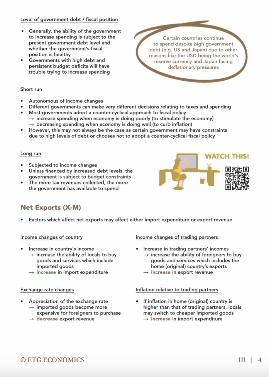
Short Run: Government expenditure is generally autonomous of income changes in the short run. Various governments worldwide, driven by different political ideologies and fiscal policies, adopt divergent strategies for managing their expenditures in response to the economic climate. A common strategy is a counter-cyclical fiscal policy, where governments increase spending during economic downturns to stimulate demand and decrease spending when the economy is booming to cool off and control inflation. It's worth noting that this isn't a one-size-fits-all approach—specific governmental or economic circumstances might warrant a different course of action.
Long Run: Government expenditure becomes more sensitive to income changes over a longer horizon. With the constraint of its budget, a government's spending potential is tied to its tax revenue—when tax collections are high, it has more money to disburse. However, this isn't a hard rule. Government spending can still be financed by debt, essentially borrowing against future income.
Government Debt / Fiscal Position: Beyond the dynamics of the economic cycle, a government's financial health plays a significant role in determining its expenditure. A government mired in high debt levels or grappling with persistent budget deficits will struggle to increase spending without risking fiscal instability or a loss of investor confidence.
Net Exports (X-M)
Net exports, defined as a nation's total exports (X) minus its total imports (M), play a crucial role in a country's aggregate demand. Various factors can influence net exports by affecting the demand for a nation's exports or imports within the nation.
Domestic Income Changes: When domestic income levels increase, citizens generally have more disposable income. This increased purchasing power often leads to a rise in demand for goods and services, which includes imports. Consequently, increased domestic income can result in reduced net exports due to increased imports. Conversely, a decline in domestic income, potentially due to an economic recession, reduces purchasing power and import demand, increasing net exports.
Income Changes of Trading Partners: The income levels of a nation's trading partners also significantly impact net exports. When these trading partners experience income growth, their demand for goods and services increases, potentially leading to more imports from the home nation and thus increasing its exports. Hence, increasing trading partners' incomes could increase the home nation's net exports. However, suppose a trading partner experiences an economic downturn and decreases their income. In that case, their import demand may fall, negatively impacting the home nation's exports and reducing its net exports.
Exchange Rate Changes: The home nation's currency exchange rate is vital to net exports. If the nation's currency appreciates, making its goods more expensive internationally, foreign export demand will likely decrease, reducing net exports. Conversely, if the nation's currency depreciates, its goods become cheaper on the international market, potentially increasing demand for its exports and hence increasing net exports.
Inflation Relative to Trading Partners: Lastly, the inflation rate relative to trading partners can also impact net exports. Suppose the home nation's inflation rate is higher than its trading partners. In that case, its goods become relatively more expensive, leading to reduced demand for its exports and increased demand for cheaper imported goods, reducing net exports. On the other hand, if the nation's inflation rate is lower than its trading partners, its goods become relatively cheaper, potentially increasing demand for its exports and decreasing demand for more expensive imported goods, thereby increasing net exports.
1.2 What is Aggregate Supply (AS)?
Aggregate Supply (AS) is the total supply of goods and services that producers in an economy are willing to offer at various price levels. AS is divided into two parts:
Short-Run Aggregate Supply (SRAS): The relationship between the price level and the quantity of goods and services produced in the short run.
Long-Run Aggregate Supply (LRAS): The total output of goods and services when the economy is at full capacity.
Real-World Example:
Investment in technology or education can shift the LRAS curve to the right. For example, Singapore's continued investment in AI and automation will increase its long-term production capacity, shifting the LRAS to the right.
2. Diagrams of Aggregate Demand and Aggregate Supply
2.1 Drawing the Aggregate Demand (AD) Curve
The AD curve slopes downward from left to right. This indicates that as the price level decreases, the quantity of goods and services demanded increases. This negative relationship exists because consumers and businesses are more likely to spend when prices are lower.
Diagram Explanation:
The vertical axis represents the price level.
The horizontal axis represents real GDP/output.
As the price level decreases, people have more money to spend on goods and services, shifting the AD curve to the right.
Real-World Example:
When the price of oil decreases, the cost of transport and production falls. This leads to lower prices for many goods and services, which, in turn, increases consumption and investment, shifting the AD curve to the right.
2.2 Drawing the Aggregate Supply (AS) Curve
There are two types of Aggregate Supply curves:
Short-Run Aggregate Supply (SRAS): This curve is upward sloping, showing that as prices rise, firms are willing to produce more due to higher profits.
Long-Run Aggregate Supply (LRAS): The LRAS curve is vertical at the economy's natural output level, which is determined by the availability of resources, technology, and capital.
Diagram Explanation:
The SRAS curve slopes upwards, indicating that higher prices incentivize firms to increase output.
The LRAS curve is vertical, as the total output remains constant at full employment.
Real-World Example:
A supply shock, such as a natural disaster disrupting production, could shift the SRAS curve left, causing a decrease in output and a rise in prices in the short run.
2.3 SRAS
Several factors can influence the position and shape of the SRAS curve:
Changes in Oil Prices: As oil is a critical input for many industries, changes in oil prices significantly impact production costs. An increase in oil prices can cause the SRAS curve to shift leftwards, indicating that firms produce less at every price level due to higher costs. Conversely, decreasing oil prices reduces production costs, causing the SRAS curve to shift rightwards.
Changes in Raw Material Prices: Similar to oil prices, fluctuations in the costs of raw materials impact production costs and hence the quantity of goods firms are willing to supply. For example, a spike in steel prices would increase costs for car manufacturers, shifting the SRAS curve to the left.
Changes in Wages: If wages rise without a corresponding increase in worker productivity, this implies higher costs for firms and results in a leftward shift of the SRAS curve. On the other hand, if wages fall or productivity rises faster than wages, this reduces costs and shifts the SRAS curve to the right.
In other words, when we have changes in the prices of factor inputs with no bearing on the productivity or productive capacity in the economy, we expect a shift in the SRAS.
2.4 LRAS
Changes to the LRAS occur due to factors that impact the economy's productive capacity:
Technological Advancements: Technology enhances productivity, allowing firms to produce more with the same resources. Therefore, technological advances can shift the LRAS curve to the right, symbolising an increase in the economy's potential output.
Changes in Productivity: Increasing education or skills training improves worker productivity, which can increase the economy's productive capacity. This factor would shift the LRAS curve to the right.
Availability of Factor Inputs: Increases in the availability of resources used in production can also increase the economy's productive capacity. For instance, the discovery of new oil reserves would lead to an increase in the LRAS, indicating a potential increase in output.
3. Shifts in the Aggregate Demand and Aggregate Supply Curves
3.1 Factors that Shift the AD Curve
The AD curve shifts when any of the four components (C, I, G, or NX) change. For example, changes in consumer confidence, government fiscal policies, or interest rates can shift the curve.
Real-World Example:
If the Singapore government cuts taxes, consumers and businesses will have more disposable income. This increase in consumption (C) and investment (I) causes the AD curve to shift to the right.
3.2 Factors that Shift the SRAS Curve
The SRAS curve shifts due to changes in production costs, wages, or technology. For example, a decrease in the cost of raw materials or wages can increase the quantity of goods and services produced, shifting the SRAS curve to the right.
Real-World Example:
A decrease in wages, as seen in certain labor market reforms, can reduce production costs, allowing businesses to produce more at lower prices, shifting the SRAS curve to the right.
3.3 Factors that Shift the LRAS Curve
The LRAS curve shifts when there are changes in the factors of production, such as technology, capital, or labor. These shifts usually occur over the long term.
Real-World Example:
Investments in education or automation (like Singapore’s AI initiatives) can increase an economy’s potential output, shifting the LRAS curve to the right.
4. Full Employment and Its Implications
4.1 What Does Full Employment Mean?
Full employment occurs when all available resources are fully utilized, but there will still be some natural unemployment due to frictional or structural factors (e.g., people between jobs or transitioning to new sectors). It is a state where the economy operates at its potential output level.
Real-World Example:
Singapore maintains low unemployment rates due to policies focused on skills development and job matching. This helps the economy operate near full employment, where production is efficient.
4.2 Near Full Employment and Its Implications
When the economy is near full employment, it operates close to its potential output, but there may still be small gaps in the labor market. This can lead to mild inflation as demand for workers exceeds supply in certain sectors.
Real-World Example:
In 2018, Singapore’s economy was near full employment. This led to concerns about wage inflation in sectors with labor shortages, especially in technology and healthcare industries.
4.3 At Full Employment
At full employment, the economy is producing its maximum sustainable output. Any further increase in demand will result in inflation, not increased output.
Real-World Example:
When the U.S. economy reached full employment before 2007, demand-side policies (like increasing government spending) led to higher inflation without an increase in real output, signaling that the economy had reached its full potential.
5. Conclusion
The Aggregate Demand and Aggregate Supply (ADAS) framework is essential for understanding macroeconomic phenomena such as inflation, unemployment, and economic growth. By grasping the shifts in AD, SRAS, and LRAS, as well as understanding the implications of full employment, students will be able to analyze how economies adjust to changes in policy and external shocks. Mastery of these concepts is crucial for anyone pursuing A Level Economics tuition or economics tuition.
Discussion Questions
What factors can cause shifts in the AD curve, and how do these shifts impact the overall economy?
How do SRAS and LRAS differ in terms of short-term and long-term economic changes?
How does full employment affect inflation and the ability to increase national output?
Can you think of a situation where an economy shifted from being near full employment to full employment?
If you're looking for top-quality economics tuition Singapore, look no further than ETG Economics Tuition. Led by Mr. Eugene Toh, who holds double Master’s degrees and has been featured in major media outlets, ETG offers specialized programs in A Level Economics tuition and IB Economics tuition. With a proven track record of success, 71% of ETG’s A Level Economics students in 2023 achieved an 'A' grade, and over 90% of students from top junior colleges, such as Raffles Institution, Hwa Chong Institution, and National Junior College, scored an 'A'. At ETG, students not only benefit from expert guidance but also gain access to in-house publications, comprehensive curricula, and exclusive resources like the Essay and CSQ Booster course. Whether you prefer face-to-face or online economics tuition, ETG provides flexibility, ensuring that students can thrive in their studies regardless of their schedules.
At ETG Economics Tuition, we are committed to helping you achieve your academic goals. Our flexible learning options, including blended learning and private econs tuition, ensure that every student can find the right path for their learning style. With personalized consultations with Mr. Toh, premium learning resources, and accurate exam predictions, ETG sets students up for success. To learn more about the ETG programme, or to register for a trial lesson, visit here. If you're ready to take the next step in your economics education, explore our programs and secure your spot with top economics tuition at ETG today!
Take a look at our stunningly curated textbooks, exclusively available for ETG students only: